Thank you Ira! His contribution to Apollo memorabilia for the May meeting was a terrific Lego Saturn V rocket. Mine was ordered from Amazon that very night. It was kept boxed up as a secret until we were into our weeks at the beach, then built with my grandsons. Bag by bag, #1 through #12, and step by step, #1 through #336, all 1969 pieces (cute, huh?) were assembled. Had to hold Sawyer, age 6, back a bit to give Evan, 4, his turns, but both boys did an excellent job. We were all very impressed with their meticulous diligence and their attention span. They stayed focused and eager for over an hour that first day. Each day after, they came to me and asked to do another bag or two. Packaged that way, multiples of any type piece clearly represent an error, so corrections are easily made. It’s not always clear how sub-assemblies go together, though, so there were a few instances of disassembly to adjust components found to be ninety degrees out of registry.
In the end, we were all justifiably proud of our work, but then the question arose of how to get it home intact. All the cars were overloaded with stuff, so there was no space to lay it out gently cradled on a quilt. Cling wrap to the rescue! It was almost like shrink wrap, and some packaging tape longitudinally over the wrap assured against disconnection of the stages. Fins removed, it slid perfectly into a box that had brought down a beach umbrella. Home safe, the wrapping cut away, the rocket now stands protected but accessible in a place of honor. Yeah, it’s in my house.
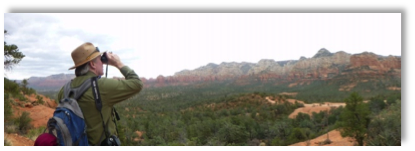
A few nights before we started on the rocket, the Moon was a few nights before full, so it was up before sunset and, more importantly, before bedtime. My little Tele Vue 85 was set up on the deck, and the boys had their first ever telescope look at the Moon. It was a good lesson for me, because the high power crater and mountain view at the terminator that I thought would be impressive did not work for them. With no observing experience, that perspective made no sense. The desired aha moment was not achieved until I switched to a medium power eyepiece that gave them a whole Moon view. That was familiar, just lots bigger and more detailed. It’s so fulfilling to watch their faces light up with smiles and hear the “Wow!” when they actually ‘get’ it!
We show globular star cluster M13 a lot at the Observatory. AKA NGC 6205 and “the Great Hercules Cluster,” it’s just always up there. It’s viewable from April to November, our whole Public Night season. It’s one of the brighter deep sky objects, +5.78 visual magnitude and 23,000 light years away, according to Sky Safari. It’s available unless clouds or the Moon overwhelms it. Only one other globular is brighter, but M22 is in Sagittarius, viewable only June through August, and never much out of the weeds. We still like showing M13 to our guests, and the Ultrastar throws a great image up on the monitor, but for me, it’s become kinda “meh.”
Until last night. I had my SCT set up in the driveway, right next to an obscenely bright street light that stays on all night. I wanted Jupiter to collimate a RACI finder and laser I just added to the tube, and to get it in the back yard I’d be way out in the wet grass. Nah, I’ll shield my eyes.
Got the hardware aligned pretty quickly and put in the ASI224MC camera but couldn’t get any image. Realizing I have no idea where focus should be so I need a bunch more preliminary work, out with the camera and back in with the diagonal and eyepiece. Gazed at binary Mizar a bit, then remembered M13 was also at the zenith on Friday night and jogged over.
Wow. Like, what? How come it looks so detailed, so interesting? It’s just M13, but most of the stars are distinct, and golden ones, sparkling more brightly and feeling closer, are scattered about. I don’t think I have ever seen it looking like this in the much larger and more capable Observatory hardware. The view was captivating. It was like someone had turned on or tuned up my non-existent adaptive optics. Or maybe there was some kind of hole in the atmosphere above me. I had first looked through the Radian 18 mm, at 130X, and the view with the Nagler 6 11 mm at 214X was just as spectacular. Tried the 9 mm but that one dulled it a bit without adding to the depth, so 261X was apparently too much magnification for the seeing.
Pretty soon I quit pondering the how or why and just reveled in the sight. Found the wife still awake, reading, and brought her out. She was not as impressed as I. Oh well, over to Jupiter for her peek, then back.
It was almost 11 when I saw a neighbor’s TV go on, so I knew someone was awake. I tiptoed over and timidly rang the doorbell. He looked at me very sideways as I explained the invitation, but he and his son-in-law both came over to look. They had some trouble seeing M13 with the streetlight competing, but they also aren’t practiced at studying DSOs. Jupiter was a much bigger hit, and tiny Saturn, up by then, really blew him away. They both thanked me vigorously, and he was still exclaiming about it as he walked home.
That’s really where it’s at, isn’t it? I had a thrilling experience, but it wasn’t enough to just enjoy it by myself. I had to try to share it. Okay, so they didn’t catch the thrill I did, but they caught one of their own.
I drove for seven hours to see a radio telescope. Green Bank is in West Virginia, passing through a forest to reach a middle of nowhere valley surrounded by mountains. This is also an isolated place in terms of being a radio free zone. There are no cell phone towers in a radius of fifty miles. This allows the telescopes to capture the radio waves coming out of space. This helps in exploration of astronomical objects like distant stars, galaxies, black holes etc. To accomplish these goals, it is important to stay away from man made radio noise.
Astronomy traditionally has been confined to seeing the light emitted by heavenly bodies. Nineteenth century discoveries proved that light is only a small part of the spectrum of what is known as electromagnetic radiation. It was found later that infrared rays (heat), x-rays, ultra violet rays, gamma rays, microwaves, radio waves are all part of this same spectrum. Telescopes were being constructed to capture the radiation coming from outer space at different frequencies. The methods of capturing are different for different types of radiation. Radio telescopes capture the radio waves by using antennas and piping the signal to sensitive receivers study.
Starting after a full day’s work, it was late in the night by the time we reached our hotel close to Green Bank. Navigation was difficult. Assuming Google maps cannot help us due to paucity of cell phone towers, we took our handheld GPS receiver which directly receives signals from the GPS satellites in the space. Unfortunately, our hotel address could not be found in its database. We tried the cell phone as long as the signal was received. And thought of resorting to good old technology of using directions from paper. Fortunately, we were able to reach the hotel (which was kind of a rural and bucolic farmhouse) in pitch darkness. The signal from the last cell phone tower, and thereafter some magic software from Google maps carried us to our destination.
Green Bank Observatory has a group which monitors for man made noise and tries to eliminate. No microwave ovens are allowed, unless they are enclosed in a metallic cage called Faraday’s cage. This cage prevents radio waves from the oven to spread out. No digital cameras are allowed because they emit radio waves as well. I saw a smart family bringing in the good old film camera, while we were not able to take any pictures inside the observatory. Not even a fitbit watch was allowed inside.
Only diesel vehicles are used on the premises because gasoline vehicles have spark plugs which initiate the combustion. The spark plugs are known to emit radio waves. Diesel on the other hand ignites by compression. The radio receivers used in the telescopes are cooled to a few degrees above absolute zero. This is to cut out the radio noise generated by the receivers. As a result, the radio receivers don’t last for more than six months. There is a shop on the premises which constantly builds replacement receivers. It is easy to distinguish man made radio waves, which have discrete (some specific frequencies) against natural ones which have continuous frequencies. Regardless, they are very strict about minimizing man made noise.
My interest in radio astronomy was triggered by a very interesting collection of video lectures on radio astronomy by Dr. Felix Lockman who is an astronomer at Green Bank. It all started accidentally in the 1930s when Karl Jansky of AT&T Bell Labs while experimenting his radio antenna for communications that some radio waves were coming from a particular direction in the sky. This could not be man made. He found that these radio waves are coming from outside of our solar system. The picture below is a replica of Jansky’s antenna at the front of the observatory. It is only a monument, not part of a working telescope.
Replica of Karl Jansky’s radio antenna
Given below is a replica of a telescope built by another radio astronomy pioneer named Grote Reber. The dish moves up and down in vertical direction using the curves in the left and the right. The whole contraption moves on rollers in a circle on the ground. This way, the telescope can be positioned to see any specific part of the sky.It is only a monument, not part of a working telescope.
Replica of Grote Reber’s radio antenna
There are several radio telescopes inside the observatory which is an area about 1-2 miles in radius. One of the telescopes, the 85 foot radio telescope was used by Frank Drake to study for possible life outside of our planet. He established SETI (Search for Extraterrestrial Intelligence), which has since moved from NASA funded venture to a silicon valley funded one. This is where Drake came up with his famous equation for the probability of finding life elsewhere in the Universe. The conclusion is that life is not unique to Earth, but should be present in other parts of the Universe. Although we have not found any yet.
The biggest telescope is the 100 meter giant whose picture is given below. It appears small because I took all the pictures included so far with my iPad pro. No digital equipment are allowed beyond this point. Because it is about 2 miles away, it looks small.
The 100m radio telescope antenna
I now have a picture from the internet which provides a close up. The buildings in the foreground give an idea of the scale of this structure. There is a curve which helps move the telescope in the vertical direction and the whole contraption resides on rollers in a circle on the ground. It can be moved to point to any specific portion of the sky.
The 100m Green Bank Telescope, courtesy Green Bank Observatory
Huge telescopes like this one cannot be made as a single piece. Multiple panels are used, and each of them driven by a motor to correct for factors like gravity, wind, heat etc. to keep the telescope focused. Special white paint keeps the dish cool and reduces the radio antenna noise.
There are advantages of a radio telescope over optical ones. Light gets blocked by the interstellar dust, whereas radio waves just pass through. Due to this reason, clouds of hydrogen, ammonia, water vapor, organic chemicals like formaldehyde and acetic acid have been detected in interstellar space using radio telescopes, which would not have been possible using the optical telescopes. Also, the radio telescopes can be used during the daytime or during lower visibility. There is no peeping into a radio telescope. The antennas feed all the data received from the radio waves into a computer, which then converts it into a colored picture. This is pretty much how major optical telescopes are operated today.
The presence of organic chemicals in space, although no DNA or proteins have been found yet, means that life could be present in other parts of our Universe. After all, Drake may be right ! If there is any life in other parts of the Universe, it is my speculation that radio telescopes may detect it first.
To be fair to other telescopes, the hidden pictures of the distant stars and galaxies made using the radio waves, can be combined with images from the optical, the infrared and the X-ray telescopes to form a composite image in what is now termed as multi messenger astronomy.
In my day to day job, when not backfilling a brick and mortar store, I am on the road. And, yes, for me, driving from location to location is a very pleasant experience. I get to ride, sometimes, for many hours. During the last long haul I decided to put a few of my favorite books, from the library, onto my iPhone. I do on occasion, listen to ‘books on tape”. So it may not come as a complete surprise, that I have meandered thru the aural equivalent of taking the road, least traveled. Please do not mistake me for Robert Frost. I do not pine for poetry’s sake (1).
Unfortunately, as is with most human beings, the spoken word is about the least efficient way to communicate information. Clearly, me speaking to you, thru this essay, is about as effective as if I were in your presence. Too long. Too boring. And often times not completely accurate. We are creatures that learn most effectively, if immersed into a world of the visual, if only to be accompanied by the audio spectrum. Perhaps, I have waved my arms, danced by jig, and done as much chalk tossing, euphemistically speaking, to overcome the odds of my non-traditional methods of conversational writing. Drat. Too long. BOOO-RING.
Oh, a Ring! Ah yes. The audio books. Panic in Level 4 (Richard Preston). The 4% Universe (Richard Panek). Eruption (Steve Olson), and Gravity’s Engines. I didn’t make it to Eruption, and absolutely recommend Panic in Level 4. However it was about two, or so hours into Gravity’s Engines, by Caleb Scharf, when I heard an alarm go off. Go ahead, say it. It was a “ring”.
I am not going to replay hours of Scharf. Not going to happen. So I encourage you to either buy the book, or download the audio, by way of Overdrive, the app. What I recall hearing was that the well of a black hole, is pumping out relativistic electrons, and streaming outward. They carve into the void, double jets of powerful radiation. And I made a mental link. It quickly became cannon fodder for me, to consider that radiating jets, from massively dense objects can form a scaffold on which ionizing gas may accrete. And my visual construct had me seeing two vast expanding conic sections. The cones had their genesis at a white dwarf, while their nebulous gaseous outreach formed dumb-bells. Yup. M27. Dumbbell Nebula. That is a real thing. Two iotas stood in my way. Nebulae are gaseous globes of ions. And they don’t require a dance partner.
Both are poor assumptions. Planetary nebulas come in dozens of shapes and sizes. I further challenged myself to look for what was not main stream. That is, Binary stars are the key to understand planetary nebulae.
I accessed YouTube, last night. Here is the link.
I will not go any further than to state that few Planetary Nebula that you see, in the night sky, were formed by one Sol. When that is the case, that is, old Solo Mio, then the gas would have vaporized much more quickly, than you or I could have lived to see, by means of a telescopic experience. Nebulae, such as these, are so rare, that they do not last more than a thousand years. Hence, there are White Dwarfs a plenty – having dissipated off their gas clouds long before you, or I could make the trek, by means of Amateur Astronomy, in our lifetimes. However, binary star systems are the new orange. Is that that bananas are the new yellow? Or am I just plain bananas? Or is that plain Vanilla? I digress. There are two of everything. Almost.
Hopefully by now you have bypassed my pablum, and have struggled thru the audio of the IAC presentation, in the above link. What I have to contribute, hopefully not to the disappointment of Dr. Henri M. J. Boffin (ESO, Garching), is that the sibling of a White Dwarf, in the presence of a Planetary Nebula, is a gentle black hole. And upon the scaffolding of outbound radiation, I present to you, the myriad structure of ionized, and visible gas.
I wasn’t too certain of what I had heard. It was helping me to conjure up ideas of light, red-shifting form the ultra-violet to our visible spectrum.
There was a chapter that buzzed by, that discoursed relativistic velocities of electrons and its relationship to the wavelength of light.
I can’t seem to find web references, for citations.
Mostly, I have taught outreach that ultra-violet light, stemming from a white dwarf, at the center of the ring nebula, interacts with the nebula and re-radiates into the visual spectrum.
Hence, I teach the public that light that cannot be seen, from the Ring Nebula, can be seen, due to an effect of re-radiation.
When I can remember, I use a small ultra-violet flashlight source, and a string of uranium glass beads, to illustrate this re-radiation.
Now, I am considering a different approach – relativistic electrons or “local” fast moving space-time – and I am now stuck without any citations.
It would become my next essay, for my Astronomy Club – however I wanted to lean away from meta-physics, and move myself towards an information essay, with solid citations.
Take this, of course, with a grain of salt. (All the best ions are salts). That if you paid attention, during Dr. Boffin’s lecture, you would have made a quick study of the light curves of these Planetary Nebulae. And that there were periodicities noted in the data. Also, giving the devil his due, we note that there were elemental studies done, on the light spectrum, yielding exacting clues as to the nebulous neighbor of our binary star systems.
Perhaps where there is no light, there is only a hole. Look closely and find periods, with no complementary light spectrum, sans the ever present White Dwarf. Pretty binary, isn’t it, my dear Watson? That is correct, my dear Amateur. Holmes, never said this was going to be Elementary.
With the occurrence of the four tiger stripes on the Southern Region of Enceladus, we turn our cats’ eye view to the ejecta. Cassini, having done four fly-bys, and directed thru the plumes, had done her analysis. And the results are quite something to speculate on, for an Astronomer, on this fine Sunday morning.
The interaction of Saturn’s E ring, notably coats the sides of Saturn’s inner moons with grains. This is cause for hurrah, as the surface of Enceladus thus becomes anew, and refreshed, sans any other geological activity. However, hold onto your hats. Da Plume! Da Plume!
The icy jets and water, exhumed from the inner workings of Enceladus, has of course been imaged by Cassini, as far back as 2005. Ultimately, there were seven fly thru’s, directly tasting gas and ice particles. The 2015 direct dive, thru the plume, detected small silica grains, by means of the Cosmic Dust Analyzer (CDA). Author Linda Spilker, in her write up of Gas Giant Planets and review of 13 years of discovery, (Science, 14 June 2019, pp. 1046-1051), excites me with the most likely source of these less than 10 nm in size particulates originating from Enceladus’ ocean (H.-W. Hsu Nature 519, 207-210, year 2015). Hydrothermal vents.
Imagine my flurry of excitement, as my visual cortex summons National Geographic of old. Our native hydrothermal vents, seated on the sea floor, spew high temperature. And deposits ejecta to build a mound, topped with heat that life cannot withstand. Almost. I say, “almost” as surrounding the hydrothermal vent mounding, is life. Life abounds in the form of adapted worms, and crustaceans. You now know my thoughts. What I see, is now what you see. Hydrothermal vents on the ocean floor of Enceladus has life.
Hydrothermal based life forms have been brought to her, by means of tidal interactions. The squish and squeeze of her mass, produces energy that is life giving. Diving below her 26-31 km thick ice shell, and within the 10 km ocean, (Spilker et al, citing L. less et al., Science 344, 78-80, year 2014) combined with the detection of organic fragments, leaves me breathless. I struggled this morning, over toast and coffee, to share with you, my thoughts of life on another planet.
I am not bound by the principles of those that cloak themselves as the priests of science. So take a moment, and congratulate yourselves on my ignorance. That I may share with you, an unfettered view, that we are not alone, after all.
gross key frequencies found in the sound of two black holes collapsing
First, some caveats. Ok. Lots of caveats. However, they are important points to remember, prior to, while reading, and after finishing this essay.
Professor Frans Pretorius never personally produced black hole merger sounds. It may read differently, further down in the essay. I wanted to be clear, and up front, that Professor Pretorius had, however, provided me a link, for a nice sound file, made by LIGO, for the first event.
The link can be found, elsewhere in this essay. However, I’d like you to have the opportunity to leave, visit, and come on back, here it is:
Having had a little email correspondence with Professor Hughes, it is imperative to point out additional caveats, before you and I proceed further, into this essay.
It is important, not only to myself, however, to Professor Hughes, that you can trace back the files, to their origin. So, in an effort, and to not be out of context, and to insure you can learn about the original calculations, please visit the above link. Here it is, again:
When you visit the MIT webpage, please take note of the added links, on the right side of their page. There you will access the sound files, that I used. By clicking on “binaries” on the MIT web page, you will transit here:
On the above link, I sourced the below file that was described as LIGO targets:
Binary black holes, each of 50 solar masses: m=100
And by clicking on “m=100”, above, it will bring you to the below page, with a resource, innocently named, “page4_3.wav”.
Moving forward, a tad, we then access, in our essay, sound files for LISA targets:
Binary black holes, mass ratio 3:1. First, with no spin effects included: hp_nospin
And by clicking on the hp_nospin link, above, it will bring you to the below page, with a resource, innocently named, “page4_4.wav”.
Another LISA target, described as follows, was accessed by clicking on “hp_rapid“:
Binary black holes, mass ratio 3:1. Each now spins very rapidly: hp_rapid
And by clicking on “hp_rapid”, above, it will bring you to the below page, with a resource, briefly named, “page4_5.wav”.
You might be inquiring, at this point, as to why I am being so particular, in making sure the links are properly cited. Please know that it is very important for you, to trace back to Professor Hughes, as he has written me on the topic and to impress: “to learn about the original calculations, to understand the nature of the model, and to learn about the shortcomings that might be present in the models.”
The sound files that I have downloaded have additional caveats:
(a) are based on approximate models for the “true” binary black hole waveform;
(b) are sampled at a finite rate;
(c) are converted to audio formats that (probably) imply a certain degree of lossiness; and
(d) are old.
Please know that I am indebted to our AAAP Astronomy Club for hosting excellent lectures. And am hopeful that you will join with us, some day, and listen in! I am further happy to say, thank you, to Professor Frans Pretorius, for his reply, as I am to Professor Scott A. Hughes, and their Research in the Group for Astrophysical general relativity at MIT. And a special thank you, to Thea Paneth, who currently is assistant to Professor Hughes, Thea took the time to take my call, and permit me the opportunity to reach out to herself, and to Professor Hughes.
And on a more personal note, you WILL find errors in my essay analysis, as well. Perhaps I have dropped a zero, in a programming comment. Or perhaps did not adjust the sample rates, in the FFT, as you would have – to produce excellent results.
I recall my photometrics, while making a video on a targeted asteroid. It wasn’t until many weeks later, at an IOTA meeting that I discovered that light measurements require calibration on known stellar targets! I would imagine, that my brief foray into “Gross Key Frequencies”, will also take a dab at my ego, and remind me once again, that learning is always on on-going process. So, please be gentle, and keep an open mind, as you read.
Later on I will decry, that I will start the essay.
Here now is the essay. Clearly, a false start.
Yup. Back in the saddle, again. Hi Ho Silver, AWAY!!
Ok. That was fun. You ALL deserved a break!
Did you remember to pause the video, or is YouTube playing the entire series? hehe.
It was over a year ago, this past March, when I had the benefit of lecture, from Frans Pretorius, during one of our clubs’ Tuesday night lectures. A few weeks later, Professor Pretorius was present in the lecture hall, and available for questioning, just as Kip Thorn was, during a talk on LIGO. A question and answer session followed. A club member ushered me onwards to go up and ask questions. My memory kicked in.
When I was in high school, I merited the opportunity of a lecture, given by Isaac Asimov, at Columbia University. I recall, all of the students, gathering around Dr Asimov, at the lectures conclusion. It so much looked liked those students that reveled in the light of Kip Thorn, some thirty or so, years later.
I decided that I wasn’t in high school, anymore, and must make the fullest attempt at making sense of the guests lecturers that were before me. I stepped up to the plate, and asked Frans Pretorius, if I could make a graphic analysis of the interferometer readings. Having tucked my BFA in digital design, discretely in my back pocket I was all too ready to bring some art to the table, for our clubs outreach. Frans P. said, convincingly so, that the data was one dimensional. So, for me, I begged off, as this was a no-go for any design thoughts.
Then, more than a year later, and for some unknown reason, I decide to take a stroll through YouTube videos. I am about half-way thru my 4th edition text on molecular biology and saw that I had exhausted most of the videos. It still remains a hidden, locked away secret, as to why I keyed in, “Fourier Transforms”. Perhaps my mind had slid off the track, and back a few years when I was experimenting with sound capture files, and Arduino.
It wasn’t until I spoke to another club member, at UACNJ, and re-admitted myself for a second splash in Fourier Transforms, where I finally embued and imprinted that I needed to learn Fast Fourier Transforms. After all, why would someone want to wait 32 years for a calculation, where you could get the answer in minutes, instead?
Then it hit me. Apply FFT to the “Sound of Two Black Holes Colliding”, with Audio Credit to “Caltech/MIT/LIGO Lab.” The MP4 video can be found here:
What to do? I had no training. Not an inkling of how to proceed. I recalled, vaguely, that MATLAB could be used to do graphic analysis. Too expensive. I Googled for open source, software. Octave! Yes. Or rather, “no”. I wasn’t up to re-installing X-Code for Mac, and to source Github packages. The learning curve, for me at least, would have been painful.
The second runner up, which by the way is as good as it gets, is found in SCILAB.
I sourced a 100 hz, and a 250 hz tone file for analysis. These tone files can be accessed, here:
I ran thru the SCILAB sample file, where a SIN and COS were merged with noise data. And then I ran the supplied FFT on all. Decent results. Amateurish, as the peak frequencies were found at one-half their actual values. However, the results were consistent.
I ventured out to the links are in the sound files that are research in the group of Professor Scott A. Hughes. And passed a wav file from a “no-spin” binary and then a “spin”, binary example.
And then downloaded then Hanford/Ligo MP4 video, and separated out the audio file. And saved it as MP3. Then converted it to WAV.
FAILURE. All zeros. A flat liner. Dead in the water.
I remember when I first produced an Arduino Cloud Height detector. And the heights were definitely off. It took a half day to realize that I had left out a zero. All fixed, and the data was shiny and new. And a three part video was published on YouTube.
I was hopeful that I wouldn’t need a half day. Maybe an hour. Off for another cup of coffee. A phone call to my friend Eric. A plea for a better conversion file.
Tic the toc.
I am a hack. I must apologize to the community at large. I took code, under my wing, and re-ordered it so that I could produce some graphs. And when the last graphic didn’t work, an hour later it would. All it took was to extend the sample size from 1000, to 10000.
Another email, shortly went out, to our math expert, Eric Leonard, saying, “all is well”. No worries.
Time to write up an essay. Here it is:
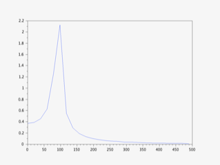
“Gross key frequencies are found in the “Sound of Two Black Holes Colliding”, with Audio Credit to Caltech/MIT/LIGO Lab.”
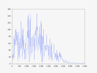
Below is my graphic FFT analysis of the Hanford MP4 file:
FFT Analysis of Two Colliding Black Holes
I converted the MP4 video to WAV format, and ran it thru code, on SCILAB.
The analysis is crude, and the peak frequencies should be doubled.
So if peaks are roughly found at 250, 500, 1300, 1700, and 2000 hz, the frequencies discovered are 500, 1000, 2600, 3400 and 4000 hz.
I apologize for intruding on your what may be your day off, from a very busy schedule. Please know that my request is certainly not of a high order. It may be perceived as an unnecessary step, into understanding the construct of a detected gravitational wave event.
It is for me, however, my second baby-step into the depth of your understanding. And I thank you for your time, today.
I have had the pleasure of listening to you twice, Professor. Once at our Princeton’s Amateur Astronomy Groups lecture at Peyton Hall, over a year ago, during April 2018. There our club had the opportunity to embrace your computational science and programming contribution to gravitational wave detection. And once again, a short while thereafter, at a Princeton sponsored lecture Kip Thorn and yourself. There you had the misfortune of me asking, as a novice, after the lecture, to describe the dimensions of the audio files waveform. There you had the happenstance to answer this novice, that the waveform was one dimensional. I had the thought that I could provide a graphic view, of the architecture of the waveform, however learning from you, first-hand, I decided that was not possible. This one dimension construct left little for this graphic artist to interpret.
Today, I stumbled upon a YouTube video, that briefly educated me on a subject that had long escaped my ability to comprehend. It was on Fourier Transforms. I had employed others programming techniques, while learning how to deploy micro-controllers in audio sampling. And Fast Fourier Transformations (FFT) were at the crux of the code. Loosely, then, I had some idea of what a microphone would pick up – as “one-dimension” could be analyzed by the FFT, and decode the population of separate frequencies. That hyperbole was subsequently lost on me, as I drifted to other subjects of interest, namely Astronomy, and microscopy.
Having had my noggin refreshed with ideations of Fourier analysis, and having visited a page, or few on LIGO, this July 4th morning, I was going to ask a friend of mine, to assist me in passing the data, from the first LIGO detection of a gravity wave, thru a Fourier transform, and list the individual frequencies, therein.
My friend, Eric Leonard, would likely jump on the chance opportunity to teach me more math. I did not want a shameful repeat of something that you have already accomplished. Would it be possible for you to direct me to the web resource page, where you have listed the separate component frequencies, analyzed by a Fourier Transform, for the peak observation of the first LIGO detection?
I would then incorporate the listed frequencies into an essay, to be published for my club’s next newsletter. In essence, I wanted interested readers to know that the audio file, from LIGO’s first detection, had a complex flavor of a multitude of embedded frequencies.
I completely understand that in the data, there are injections or glitches that may reside within. However, as an Amateur, and essayist, (a poor one at that!) I am more interested in writing about how the next young mind could embrace this analysis. Hopefully, an essay would spark young minds, or even those a little older, to embrace some of the complexities of your work, and to dig a little deeper into the literature of gravity waves, black holes, neutron stars, their collapse and signature events, as recorded by LIGO. And in doing so, enrich my learning, and shorten my learning curve at tad, at my next Astronomy outreach.
Professor Pretorius, once again, if you already have the frequencies listed, for the time period of the detection that you had constructed for the audio presentation, that would be wonderful.
I am hopeful that some basic viewpoint, into the art, of the structure of the frequencies, if only superficially on my part, would provide another viewport into the fingerprint of the first detection. And become a base of discussion for minds, both young and old that come out to the events that I out-reach to, for Astronomy. In particular, an enlightening others and leading them to understanding gravitational collapse.
Thank you so very much,
Ted Frimet
Of course, you all know the results. They are printed above. If you want to take a peek, under the sheets, and see what 6 hours of study can yield, then venture forth, you brave souls:
y=wavread(“/Users/theodorefrimet/ligo20160211v2.wav”,[1 10000]) //the first 10000 samples
q=fft(y);
//plot(q);
sample_rate=10000;
t = 0:1/sample_rate:.05;
N=size(t,’*’); //number of samples
f=sample_rate*(0:(N/2))/N; //associated frequency vector
n=size(f,’*’)
plot(f,abs(q(1:n)))
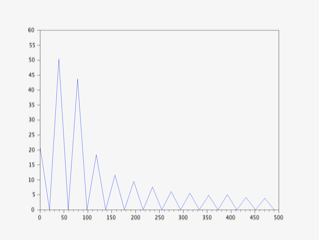
Below is a synopsis of the work that I did, for the past few hours, with the bottom graph being my failure, until I adjusted the sample size.
I installed SCILAB into my Mac, and hacked to produce the below code.
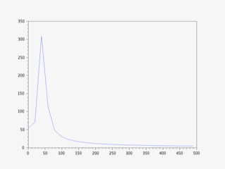
The sound file is a 30 second WAV of 250Hz
y=wavread(“/Users/theodorefrimet/250Hz_44100Hz_16bit_30sec.wav”,[1 1000]) //the first 1000 samples
q=fft(y);
//plot(q);
sample_rate=1000;
t = 0:1/sample_rate:.05;
N=size(t,’*’); //number of samples
f=sample_rate*(0:(N/2))/N; //associated frequency vector
n=size(f,’*’)
plot(f,abs(q(1:n)))
It produced this graph, which appears to peak at [one-half] the hz of the sound file:
Here is my Octave program…
Eric Leonard has re-written the code for Octave, so that we get a proper result for the 250 Hz file.
cd c:\EricFiles\Astronomy\TedFiles
y = load(‘250Hz_44100Hz_1000Samps.txt’);
q=fft(y);
% plot(q);
sample_rate=44100;
N=length(y);
f=sample_rate*(0:(N/2))/N; % associated frequency vector
n=length(f);
plot(f,abs(q(1:n)), ‘b-x’)
axis([0 400 0 300]) % to obtain the magnified view
grid on
If you follow that lead, with Octave, or with Matlab, your results will be precise.
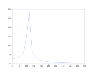
I re-tested on a 30 second WAV of 100 Hz:
It appears to me that the “peak” from the FFT, is identifying the key “frequencies” at [frequency/2].
Going forward, I downloaded a sample audio file, from MIT.
It was produced by Professor Scott A Hughes.
The naming conventions were a tad basic.
The WAV file is for two binary black holes, with 50 solar masses, each, so the total mass = 100!
I downloaded that target file, and processed it using SCILAB, and FFT.
Below is the graphic that resulted:
Am I off my bird, or is the above 100 kHz * 2 = 200 kHz frequency for Professor Hughes sample?
Then, I downloaded the “no-spin” binary example:
and finally the “spin” binary examples:
And here is MY FAILURE. I downloaded the Hanford/Ligo MP4 video, and separated out the audio file. And saved it as MP3. Then converted it to WAV.
Here is the code:
y=wavread(“/Users/theodorefrimet/ligomp3.wav”,[1 1000]) //the first 1000 samples
q=fft(y);
//plot(q);
sample_rate=1000;
t = 0:1/sample_rate:.05;
N=size(t,’*’); //number of samples
f=sample_rate*(0:(N/2))/N; //associated frequency vector
n=size(f,’*’)
plot(f,abs(q(1:n)))
Nasa puts up deep-space atomic clock
Nasa has put a miniaturised atomic clock in orbit that it believes can revolutionise deep-space navigation. Nasa has put a miniaturised atomic clock in orbit that it believes can revolutionise deep-space navigation. The timepiece was one of 24 separate deployments from a Falcon Heavy rocket that launched from Florida on Tuesday…more
Lovell Telescope -BBC
Jodrell Bank gains Unesco World Heritage status
It has been at the forefront of astronomical research since its inception in 1945 and tracked US and Russian craft during the space race. It joins the ancient Iraqi city of Babylon and other locations that have been added to the prestigious list…more
Spektr-RG -BBC
Spektr-RG: Powerful X-ray telescope launches to map cosmos
One of the most significant Russian space science missions in the post-Soviet era has launched from Baikonur.
The Spektr-RG telescope is a joint venture with Germany that will map X-rays across the entire sky in unprecedented detail…more
-Adobe Stock
Solving the sun’s super-heating mystery with Parker Solar Probe
It’s one of the greatest and longest-running mysteries surrounding, quite literally, our sun — why is its outer atmosphere hotter than its fiery surface?
University of Michigan researchers believe they have the answer, and hope to prove it with help from NASA’s Parker Solar Probe…more
Chandrayaan-ISRO
Chandrayaan-2: India launches second Moon mission
India has successfully launched its second lunar mission a week after it halted the scheduled blast-off due to a technical snag. Chandrayaan-2 was launched at 14:43 local time (09:13 GMT) from the Sriharikota space station. India’s space chief said his agency had “bounced back with flying colours” after the aborted first attempt…more
-NASA
Nasa Moon lander vision takes shape
Nasa has outlined more details of its plans for a landing craft that will take humans to the lunar surface. The plans call for an initial version of the lander to be built for landing on the Moon by 2024; it would then be followed by an enhanced version…more
-OGLE/Warsaw Univ.
Milky Way galaxy is warped and twisted, not flat
Our galaxy, the Milky Way, is “warped and twisted” and not flat as previously thought, new research shows. Analysis of the brightest stars in the galaxy shows that they do not lie on a flat plane as shown in academic texts and popular science books…more
-SyFy
An amateur astronomer has discovered a nearby galaxy
I am a big supporter of amateur astronomy for a lot of reasons. First, it gets people outside and looking up, which is just a good thing to do. It also fosters an appreciation for the sky and the beauty in it. I consider myself an amateur astronomer, too…more
by Rex Parker, Phd director@princetonastronomy.org
June 11 Meeting (7:30pm) – at the NJ State Museum Planetarium. We’ve come to the last meeting of our “academic” season, to be held at the NJ State Museum Planetarium in Trenton. The museum is located at 205 W State Street next to the NJ State House (gold dome). Park in the lot at the bottom of the hill behind the museum next to the planetarium dome. See Ira’s section in this issue for program information.
Galaxies of Late Spring. It’s not too late to observe some of the Virgo-Coma supercluster of galaxies through telescopes this month. This gigantic grouping of galaxies spans about 15 million light years with approximate center about 60 million light years away. Dozens of the larger and higher brightness magnitude galaxies in this group can be seen in telescopes with 8-16 inch mirrors, such as the Celestron-14 at the AAAP observatory in Washington Crossing State Park. The view angles presented by different galaxies range from edge-on to face-on, which along with distance greatly affect surface brightness and aspect ratio in the telescope. One of the prototypical face-on galaxies in the Virgo group is Messier 100 (M100), a beautifully structured spiral about 50 million light years away from us. The image below is processed from about 45 hours of CCD data (luminance, red, green, and blue) for M100 acquired by remote astrophotography using a 16-inch telescope at Cerro Tololo in the Chilean Andes. The final image shows M100’s distinct morphology and predominantly blue color with patches of glowing red ionized hydrogen H-II regions of new star formation. As discussed at recent meetings, visual observing through the eyepiece won’t reveal these colors due to low light level constraints in human eye physiology. Still, many observers subjectively feel a profound cosmological sensation from seeing spiral galaxies like M100 in a telescope eyepiece.
Messier 100, spiral galaxy in the Virgo-Coma Supercluster. Image by Rex Parker using the 16-inch PROMPT2 telescope from Cerro Tololo, Chile (Star Shadows Remote Observatory).
Skynet Project Renewal. Good news! AAAP has renewed the contract with Skynet for another two years. Two years ago we began a project to bring access to remote astrophotography to AAAP members. Skynet is the brainchild of Dr Dan Reichart of the Physics and Astronomy Dept at the University of North Carolina, Chapel Hill. The internet-based queue scheduling program runs on a computer at UNC which accesses a system of observatories created for remote imaging. This system, the Skynet Robotic Telescope Network, comprises more than a dozen telescopes around the world at observatories in Chile, Australia, Italy, Canada, and US. Each telescope is set up with robotic tracking mount, CCD camera, and filters for remote color image acquisition. Tutorial videos are available to help a user get up and running. For further background read my article in the June 2017 issue of Sidereal Times available from the AAAP website archive.
Whether you’re a first-time astronomer or seasoned observer, Skynet’s easy-to-use yet powerful interface allows you to get images of celestial objects from the Messier and NGC deep sky catalogs. Skynet also includes a basic image processing program “Afterglow” that runs on the server, so you don’t need any special software on your PC. You also can download and process your images locally with your own programs like CCD Stack or Maxim DL if you like. While there are limits on the length of exposures, Skynet is a great way to get onto the learning curve for astro-imaging and understanding how the modern practice of astronomy works. Current AAAP members who have used the system will have new credits added to their accounts. If you are interested in access to Skynet send me an e-mail note to get a new user account.
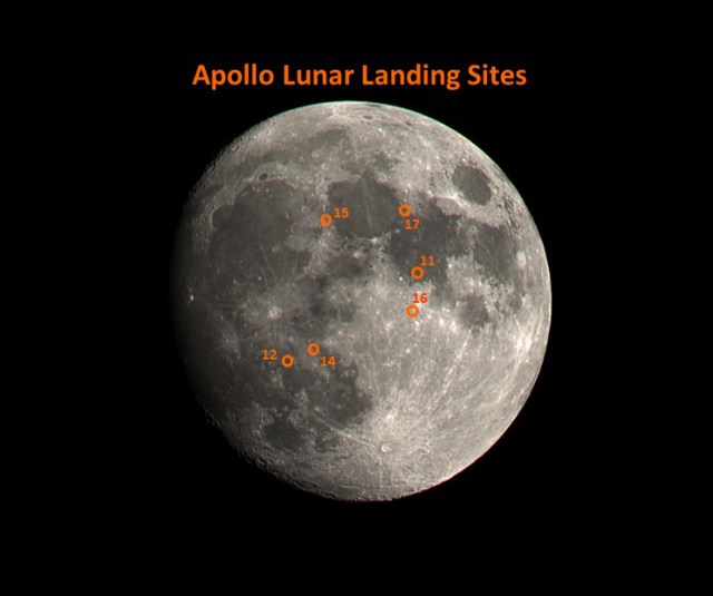
The Moon in All It’s Glory. Celebrating the achievements of the Apollo program will reach a crescendo this summer for the 50th anniversary of the Apollo 11 landing in July. With kudo’s to our May speaker, James Chen (author of How to Find the Apollo Landing Sites, published by Springer), I took the liberty of assembling a composite of all the lunar landing sites on an image of the nearly full moon I took a couple years ago with a small refractor telescope. One of many remarkable aspects of the landings is how close together they were in both time and space on the moon’s surface. Only a small fraction of the landscape was sampled by the 6 locations. All the landings were done in less than 3-1/2 years, a feat that seems impossible today.
Recently, a fellow board member of Astronomy and Science Club from my retirement community brought to my attention an intriguing New Jersey site. Though, at the time of this writing, I have not had an opportunity to visit it myself, I thought its existence should be brought to the attention of the AAAP membership.
I called the InfoAge Space Exploration Center, ISEC, located at 2300 Marconi Rd in Wall Township, NJ and found that the Center sports the TLM-18, a 60 foot operational radio telescope. This telescope was refurbished by a team from the Info Center and Princeton University. It is currently used to detect radio signals from the Milky Way. Center visitors can see the telescope in use and discuss its galactic data gathering with its operators.
If you should get to see the Center and the TLM-18 soon, please let me know what you think about both. The ISEC is open to the public on Wednesday, Saturday and Sunday from 1:00 PM to 5:00 PM. Admission costs are $5.00 per person.
In addition, at the last meeting of the Board of Directors, I assumed the responsibility for managing the AAAP “Meet Up” account. This means that I will be listing and updating all relevant events in which our club will be participating. So, if you have a Meet Up account, stay tuned. If not, open one to stay abreast.
The June meeting of the AAAP, and our last until next September, will take place on June 11th at the Planetarium of the New Jersey State Museum in Trenton. The meeting starts at 7:30 PM.
In addition to our regular club meeting, attendees will view the latest show CAPCOM GO! The Apollo Story. “One small step…” From the producers of the award-winning fulldome shows ‘We Are Stars’ and ‘ASTRONAUT’ comes ‘CAPCOM GO! The Apollo Story’. An immersive, historical documentary that showcases the achievements of the Apollo program and what it took to put the first human on the Moon. It introduces a new generation to the immense challenges they overcame and will inspire them to become the explorers, designers, engineers, thinkers and dreamers of the future.
There is plenty of parking in front of the planetarium entrance behind the museum. Museum is located at –205 W. State Street, Trenton, NJ 08625.
If you are registered for the Celestial Navigation class on June 15-16 you will receive an email from me with the latest details this weekend (June 1-2). If you believe you are registered and do not get this email please contact me at program@princetonastronomy.org


 Messier 100, spiral galaxy in the Virgo-Coma Supercluster. Image by Rex Parker using the 16-inch PROMPT2 telescope from Cerro Tololo, Chile (Star Shadows Remote Observatory).