
by Theodore R. Frimet
gross key frequencies found in the sound of two black holes collapsing
First, some caveats. Ok. Lots of caveats. However, they are important points to remember, prior to, while reading, and after finishing this essay.
Professor Frans Pretorius never personally produced black hole merger sounds. It may read differently, further down in the essay. I wanted to be clear, and up front, that Professor Pretorius had, however, provided me a link, for a nice sound file, made by LIGO, for the first event.
The link can be found, elsewhere in this essay. However, I’d like you to have the opportunity to leave, visit, and come on back, here it is:
https://www.ligo.caltech.edu/video/ligo20160211v2
Frans Pretorius notes that Scott Hughes, at MIT, has made sound files from simulated events that last longer. Visit them, here:
http://gmunu.mit.edu/sounds/sounds.html
Having had a little email correspondence with Professor Hughes, it is imperative to point out additional caveats, before you and I proceed further, into this essay.
It is important, not only to myself, however, to Professor Hughes, that you can trace back the files, to their origin. So, in an effort, and to not be out of context, and to insure you can learn about the original calculations, please visit the above link. Here it is, again:
http://gmunu.mit.edu/sounds/sounds.html
When you visit the MIT webpage, please take note of the added links, on the right side of their page. There you will access the sound files, that I used. By clicking on “binaries” on the MIT web page, you will transit here:
http://gmunu.mit.edu/sounds/comparable_sounds/comparable_sounds.html
On the above link, I sourced the below file that was described as LIGO targets:
Binary black holes, each of 50 solar masses: m=100
And by clicking on “m=100”, above, it will bring you to the below page, with a resource, innocently named, “page4_3.wav”.
Moving forward, a tad, we then access, in our essay, sound files for LISA targets:
Binary black holes, mass ratio 3:1. First, with no spin effects included: hp_nospin
And by clicking on the hp_nospin link, above, it will bring you to the below page, with a resource, innocently named, “page4_4.wav”.
Another LISA target, described as follows, was accessed by clicking on “hp_rapid“:
Binary black holes, mass ratio 3:1. Each now spins very rapidly: hp_rapid
And by clicking on “hp_rapid”, above, it will bring you to the below page, with a resource, briefly named, “page4_5.wav”.
You might be inquiring, at this point, as to why I am being so particular, in making sure the links are properly cited. Please know that it is very important for you, to trace back to Professor Hughes, as he has written me on the topic and to impress: “to learn about the original calculations, to understand the nature of the model, and to learn about the shortcomings that might be present in the models.”
The sound files that I have downloaded have additional caveats:
(a) are based on approximate models for the “true” binary black hole waveform;
(b) are sampled at a finite rate;
(c) are converted to audio formats that (probably) imply a certain degree of lossiness; and
(d) are old.
Please know that I am indebted to our AAAP Astronomy Club for hosting excellent lectures. And am hopeful that you will join with us, some day, and listen in! I am further happy to say, thank you, to Professor Frans Pretorius, for his reply, as I am to Professor Scott A. Hughes, and their Research in the Group for Astrophysical general relativity at MIT. And a special thank you, to Thea Paneth, who currently is assistant to Professor Hughes, Thea took the time to take my call, and permit me the opportunity to reach out to herself, and to Professor Hughes.
And on a more personal note, you WILL find errors in my essay analysis, as well. Perhaps I have dropped a zero, in a programming comment. Or perhaps did not adjust the sample rates, in the FFT, as you would have – to produce excellent results.
I recall my photometrics, while making a video on a targeted asteroid. It wasn’t until many weeks later, at an IOTA meeting that I discovered that light measurements require calibration on known stellar targets! I would imagine, that my brief foray into “Gross Key Frequencies”, will also take a dab at my ego, and remind me once again, that learning is always on on-going process. So, please be gentle, and keep an open mind, as you read.
Later on I will decry, that I will start the essay.
Here now is the essay. Clearly, a false start.
Yup. Back in the saddle, again. Hi Ho Silver, AWAY!!
Ok. That was fun. You ALL deserved a break!
Did you remember to pause the video, or is YouTube playing the entire series? hehe.
It was over a year ago, this past March, when I had the benefit of lecture, from Frans Pretorius, during one of our clubs’ Tuesday night lectures. A few weeks later, Professor Pretorius was present in the lecture hall, and available for questioning, just as Kip Thorn was, during a talk on LIGO. A question and answer session followed. A club member ushered me onwards to go up and ask questions. My memory kicked in.
When I was in high school, I merited the opportunity of a lecture, given by Isaac Asimov, at Columbia University. I recall, all of the students, gathering around Dr Asimov, at the lectures conclusion. It so much looked liked those students that reveled in the light of Kip Thorn, some thirty or so, years later.
I decided that I wasn’t in high school, anymore, and must make the fullest attempt at making sense of the guests lecturers that were before me. I stepped up to the plate, and asked Frans Pretorius, if I could make a graphic analysis of the interferometer readings. Having tucked my BFA in digital design, discretely in my back pocket I was all too ready to bring some art to the table, for our clubs outreach. Frans P. said, convincingly so, that the data was one dimensional. So, for me, I begged off, as this was a no-go for any design thoughts.
Then, more than a year later, and for some unknown reason, I decide to take a stroll through YouTube videos. I am about half-way thru my 4th edition text on molecular biology and saw that I had exhausted most of the videos. It still remains a hidden, locked away secret, as to why I keyed in, “Fourier Transforms”. Perhaps my mind had slid off the track, and back a few years when I was experimenting with sound capture files, and Arduino.
It wasn’t until I spoke to another club member, at UACNJ, and re-admitted myself for a second splash in Fourier Transforms, where I finally embued and imprinted that I needed to learn Fast Fourier Transforms. After all, why would someone want to wait 32 years for a calculation, where you could get the answer in minutes, instead?
Then it hit me. Apply FFT to the “Sound of Two Black Holes Colliding”, with Audio Credit to “Caltech/MIT/LIGO Lab.” The MP4 video can be found here:
https://www.ligo.caltech.edu/video/ligo20160211v2
What to do? I had no training. Not an inkling of how to proceed. I recalled, vaguely, that MATLAB could be used to do graphic analysis. Too expensive. I Googled for open source, software. Octave! Yes. Or rather, “no”. I wasn’t up to re-installing X-Code for Mac, and to source Github packages. The learning curve, for me at least, would have been painful.
The second runner up, which by the way is as good as it gets, is found in SCILAB.
I sourced a 100 hz, and a 250 hz tone file for analysis. These tone files can be accessed, here:
https://www.mediacollege.com/audio/tone/download/
I ran thru the SCILAB sample file, where a SIN and COS were merged with noise data. And then I ran the supplied FFT on all. Decent results. Amateurish, as the peak frequencies were found at one-half their actual values. However, the results were consistent.
I ventured out to the links are in the sound files that are research in the group of Professor Scott A. Hughes. And passed a wav file from a “no-spin” binary and then a “spin”, binary example.
And then downloaded then Hanford/Ligo MP4 video, and separated out the audio file. And saved it as MP3. Then converted it to WAV.
FAILURE. All zeros. A flat liner. Dead in the water.
I remember when I first produced an Arduino Cloud Height detector. And the heights were definitely off. It took a half day to realize that I had left out a zero. All fixed, and the data was shiny and new. And a three part video was published on YouTube.
I was hopeful that I wouldn’t need a half day. Maybe an hour. Off for another cup of coffee. A phone call to my friend Eric. A plea for a better conversion file.
Tic the toc.
I am a hack. I must apologize to the community at large. I took code, under my wing, and re-ordered it so that I could produce some graphs. And when the last graphic didn’t work, an hour later it would. All it took was to extend the sample size from 1000, to 10000.
Another email, shortly went out, to our math expert, Eric Leonard, saying, “all is well”. No worries.
Time to write up an essay. Here it is:
“Gross key frequencies are found in the “Sound of Two Black Holes Colliding”, with Audio Credit to Caltech/MIT/LIGO Lab.”
The Hanford MP4 file, is of course found for download, here:
https://www.ligo.caltech.edu/video/ligo20160211v2
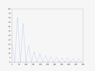
Below is my graphic FFT analysis of the Hanford MP4 file:
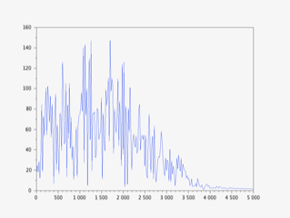
FFT Analysis of Two Colliding Black Holes
I converted the MP4 video to WAV format, and ran it thru code, on SCILAB.
The analysis is crude, and the peak frequencies should be doubled.
So if peaks are roughly found at 250, 500, 1300, 1700, and 2000 hz, the frequencies discovered are 500, 1000, 2600, 3400 and 4000 hz.
I apologize for intruding on your what may be your day off, from a very busy schedule. Please know that my request is certainly not of a high order. It may be perceived as an unnecessary step, into understanding the construct of a detected gravitational wave event.
It is for me, however, my second baby-step into the depth of your understanding. And I thank you for your time, today.
I have had the pleasure of listening to you twice, Professor. Once at our Princeton’s Amateur Astronomy Groups lecture at Peyton Hall, over a year ago, during April 2018. There our club had the opportunity to embrace your computational science and programming contribution to gravitational wave detection. And once again, a short while thereafter, at a Princeton sponsored lecture Kip Thorn and yourself. There you had the misfortune of me asking, as a novice, after the lecture, to describe the dimensions of the audio files waveform. There you had the happenstance to answer this novice, that the waveform was one dimensional. I had the thought that I could provide a graphic view, of the architecture of the waveform, however learning from you, first-hand, I decided that was not possible. This one dimension construct left little for this graphic artist to interpret.
Today, I stumbled upon a YouTube video, that briefly educated me on a subject that had long escaped my ability to comprehend. It was on Fourier Transforms. I had employed others programming techniques, while learning how to deploy micro-controllers in audio sampling. And Fast Fourier Transformations (FFT) were at the crux of the code. Loosely, then, I had some idea of what a microphone would pick up – as “one-dimension” could be analyzed by the FFT, and decode the population of separate frequencies. That hyperbole was subsequently lost on me, as I drifted to other subjects of interest, namely Astronomy, and microscopy.
Having had my noggin refreshed with ideations of Fourier analysis, and having visited a page, or few on LIGO, this July 4th morning, I was going to ask a friend of mine, to assist me in passing the data, from the first LIGO detection of a gravity wave, thru a Fourier transform, and list the individual frequencies, therein.
My friend, Eric Leonard, would likely jump on the chance opportunity to teach me more math. I did not want a shameful repeat of something that you have already accomplished. Would it be possible for you to direct me to the web resource page, where you have listed the separate component frequencies, analyzed by a Fourier Transform, for the peak observation of the first LIGO detection?
I would then incorporate the listed frequencies into an essay, to be published for my club’s next newsletter. In essence, I wanted interested readers to know that the audio file, from LIGO’s first detection, had a complex flavor of a multitude of embedded frequencies.
I completely understand that in the data, there are injections or glitches that may reside within. However, as an Amateur, and essayist, (a poor one at that!) I am more interested in writing about how the next young mind could embrace this analysis. Hopefully, an essay would spark young minds, or even those a little older, to embrace some of the complexities of your work, and to dig a little deeper into the literature of gravity waves, black holes, neutron stars, their collapse and signature events, as recorded by LIGO. And in doing so, enrich my learning, and shorten my learning curve at tad, at my next Astronomy outreach.
Professor Pretorius, once again, if you already have the frequencies listed, for the time period of the detection that you had constructed for the audio presentation, that would be wonderful.
I am hopeful that some basic viewpoint, into the art, of the structure of the frequencies, if only superficially on my part, would provide another viewport into the fingerprint of the first detection. And become a base of discussion for minds, both young and old that come out to the events that I out-reach to, for Astronomy. In particular, an enlightening others and leading them to understanding gravitational collapse.
Thank you so very much,
Ted Frimet
Of course, you all know the results. They are printed above. If you want to take a peek, under the sheets, and see what 6 hours of study can yield, then venture forth, you brave souls:
y=wavread(“/Users/theodorefrimet/ligo20160211v2.wav”,[1 10000]) //the first 10000 samples
q=fft(y);
//plot(q);
sample_rate=10000;
t = 0:1/sample_rate:.05;
N=size(t,’*’); //number of samples
f=sample_rate*(0:(N/2))/N; //associated frequency vector
n=size(f,’*’)
plot(f,abs(q(1:n)))
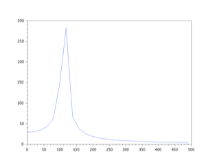
Below is a synopsis of the work that I did, for the past few hours, with the bottom graph being my failure, until I adjusted the sample size.
I installed SCILAB into my Mac, and hacked to produce the below code.
The sound file is a 30 second WAV of 250Hz
y=wavread(“/Users/theodorefrimet/250Hz_44100Hz_16bit_30sec.wav”,[1 1000]) //the first 1000 samples
q=fft(y);
//plot(q);
sample_rate=1000;
t = 0:1/sample_rate:.05;
N=size(t,’*’); //number of samples
f=sample_rate*(0:(N/2))/N; //associated frequency vector
n=size(f,’*’)
plot(f,abs(q(1:n)))
It produced this graph, which appears to peak at [one-half] the hz of the sound file:
Here is my Octave program…
Eric Leonard has re-written the code for Octave, so that we get a proper result for the 250 Hz file.
cd c:\EricFiles\Astronomy\TedFiles
y = load(‘250Hz_44100Hz_1000Samps.txt’);
q=fft(y);
% plot(q);
sample_rate=44100;
N=length(y);
f=sample_rate*(0:(N/2))/N; % associated frequency vector
n=length(f);
plot(f,abs(q(1:n)), ‘b-x’)
axis([0 400 0 300]) % to obtain the magnified view
grid on
If you follow that lead, with Octave, or with Matlab, your results will be precise.

I re-tested on a 30 second WAV of 100 Hz:
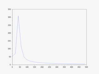
It appears to me that the “peak” from the FFT, is identifying the key “frequencies” at [frequency/2].
Going forward, I downloaded a sample audio file, from MIT.
It was produced by Professor Scott A Hughes.
The naming conventions were a tad basic.
The WAV file is for two binary black holes, with 50 solar masses, each, so the total mass = 100!
I downloaded that target file, and processed it using SCILAB, and FFT.
Below is the graphic that resulted:
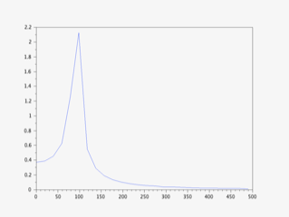
Am I off my bird, or is the above 100 kHz * 2 = 200 kHz frequency for Professor Hughes sample?
Then, I downloaded the “no-spin” binary example:

and finally the “spin” binary examples:
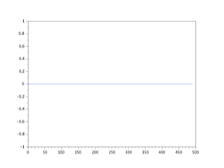
And here is MY FAILURE. I downloaded the Hanford/Ligo MP4 video, and separated out the audio file. And saved it as MP3. Then converted it to WAV.
Here is the code:
y=wavread(“/Users/theodorefrimet/ligomp3.wav”,[1 1000]) //the first 1000 samples
q=fft(y);
//plot(q);
sample_rate=1000;
t = 0:1/sample_rate:.05;
N=size(t,’*’); //number of samples
f=sample_rate*(0:(N/2))/N; //associated frequency vector
n=size(f,’*’)
plot(f,abs(q(1:n)))
Here is the ORIGINAL link to the file:
https://www.ligo.caltech.edu/video/ligo20160211v2
I get ZERO analysis out of the FFT process.
ALL the sample data that comes back, out the FFT, are zeroes.
Which of course leads to the below plot:


https://drive.google.com/open?id=1I1fyu2ooHrkcnl-WpE78zpJ9NdquwQ0K