By William H. Davis Jr.

“The Great Attractor Is Drawing the Milky Way at 1.3 Million Miles per Hour (580 km/sec) — What Does It Mean for Our Galaxy?

Learn about the Great Attractor, a region of the universe that is constantly pulling the Milky Way and thousands of other galaxies”.

Written by Jack Knudson“

“Right now, a faraway region of the universe is pulling the Milky Way and neighboring galaxies toward it. We’re technically moving at blistering speeds of around 1.3 million miles per hour in its direction, but we can’t feel this movement at all. The mysterious area that’s drawing us in, called the Great Attractor, has intrigued scientists for years.”

“This is where the Great Attractor comes in. In the 1970s, researchers noticed a significant anomaly that had materialized in a dipole pattern: The space ahead of Earth appeared hotter, while the space trailing behind appeared colder, according to the University of Southern California. Scientists have since determined that this is likely not an intrinsic effect of the Big Bang, but an illusion caused by the Solar System speeding through space.

“Regardless, one thing became clear: the Solar System — and our whole galaxy — was being pulled by some unknown force.”

“One way to envision the Great Attractor’s influence is to look at it as a hierarchy. The Local Group of galaxies, which includes the Milky Way, is at the bottom rung, being pulled toward the Virgo cluster. These two are both being pulled toward the larger Virgo Supercluster, which itself is being pulled toward the Laniakea Supercluster.”

“All this pulling comes from a central gravitational point in the Laniakea supercluster, which is attracting the aforementioned galaxy clusters due to its immense mass.

It might be hard to believe, but this isn’t even the end of the hierarchy. Scientists believe that the Laniakea supercluster is pulled by the Shapley super cluster, an even larger collection of galaxy clusters with a center that’s about 650 million light-years from Earth. In short, not even the puller is immune from being pulled.”

“Jun 4, 2026, 6:45 PM| 3 min read”

Comments: Being pulled or pushed is an incorrect description. Everything from inside an atom to large scale structures has inherent motion, which is conserved. Motion follows the gravitational terrain in orbits or freely moves if it exceeds an escape velocity. IT will move across the universal terrain between systems. The frequency shifts do to motion are not illusions.

This opens up the following observations and questions:

1. Do the spectral shifts of the 100,000 to 300,000+ galaxies in the Area of the Great Attractor compromise Hubbell’s constant? The Hubble constant is based on a statistical correlation analysis which is used to process a set of data to a linear or possibly second order relationship. The start of the model should be random to establish the base mean and STD. No cherry picking. Additional data can be added as it is discovered. It is expected that additional data over time will change the mean.  The slope or mean is only about the data not any theory or empirical physics equation result.
   
2. Special relativity requires any motion t o be described in the frame of the observer (o). No preferred observations. The description above is based on the attractor drawing Earth (o)?  To frame the system correctly, the attractor (e) is moving away from the observer on Earth. If it is moving toward Earth then it should be blue shifted. The stated shifts were derived from using the wave length ratio z.  z=(λe-λo)/λ0  = λe/λo-1    → the range of λo is  λe→∞.   This calculation is very non linear and not proportional? It cannot be mathematically accurate to calculate velocity without converting to frequency (energy). There is no law of the conservation of length. There is a law of the conservation of energy using frequency

The only proper accurate equation is the Relativistic Doppler equation which also corrects the clock differences do to the motion and combines the blue and redshift first order equations in to a single second order equation to describe the total system being studied.

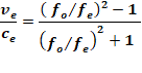
Compare using wave length or z versus frequency:

Z  Observed (qualitative) metric of increased wave length as meters as velocity increases:

1. Range observed is λ_o→ to ∞.
2. Completely non linear and non proportional. Only converts to frequency with error do to ∞ in the denominator range. It is a qualitative metric which is the inverse of energy.
3. Does not matchup with v/c an empirical linear proportional function.
4. Red shift or z originates from early observations as a rough qualitative comparison of observed objects
5. Limited, the units are meters which contain one degree of information.
6. Is not very suitable to calculate an accurate velocity.
7. 6. Not directly compatible with law of conservation of energy. No conservation of wave length.

Frequency

1. Represents energy as Planks Equation. Completely linear and proportional to velocity.
2. Range of f_o is f _e→0=1
3. Matches up with v/c  0→c  =1
4. More dimensions of information seconds and cycles (c/λ) . Represents energy.
5. Completely accurate to calculate velocity subject to clock correction at higher v.
6. Conservation of energy applies. Can be set up as an energy balance since every redshift is balanced with a blue shift on the far side observation.

Relativistic Doppler equation:

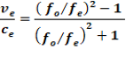
1. Combines the first order red and blueshift equations and corrects the different clock rates.
2. Is the complete description of this system of red and blue shift with a second order equation that plots in 2 quadrants +v and –v.

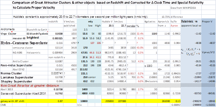
Comments:

I have noticed several different Hubble values which were used in the spreadsheet ±.05 %. The Hubble and Web telescopes have different values for objects further away. A correlation analysis of the data is only about the data. There is no law of nature involved. Unless there is proof of the correlation and it is tested, it should not be used for precise calculations. The fact that 65 galaxies in the Virgo Cluster are blue shifted makes a point. This data is not even in the same xy quadrant. The next paper admits various cherry picking, omitting closer observations and for other reasons. If the observer was in the Virgo cluster and they same thing was done etc. You would not have a very good model.  If this data is used then the model will have a high STD or variation. The mean would change. The stock market predicted seven of the last three recessions!!! In Industry we use SQC (statistical process control) to model an established process. When a 6 point trend ± compared to the mean happens, an adjustment has to be made to bring the process back to the mean. If a data point is beyond ±3 standard deviations then someone has to figure out what happened. The statistics are only about the data produced. It doesn’t tell you what’s going on

 Comments on the excerpts following paper:  some letters and words did not transfer.

The density and peculiar velocity fields of nearby galaxies Michael A. Strauss School of Natural Sciences, Institute for Advanced Study, Princeton, New Jersey 08540 and Jeffrey A Willick Observatories of the Carnegie Institute of Washington, 813 Santa Barbara Street, Pasadena, California 91101-1292

“The Hubble Law states that at distances much less than the Hubble radius, the expansion of the universe causes the recession velocity of a galaxy cz to be proportional to its distance r: cz = H0r; (1) where H0 is the Hubble Constant, whose value remains uncertain by a factor of two; in astronomer’s units, it is often written as H0 = 100h km s1 Mpc1 , the quantity h parameterizing our ignorance of its value. Mpc stands for mega parsecs, the common unit of distance for much extragalactic work: 1 Mpc = 3:08 1024 cm. Thus in physicist’s units, H0 = 3:25 1018 h sec, or H1 01010 h1 yr. In practice, we will rarely be troubled by the uncertain value of h in this review, because we will measure distances in units of km s1 , wherein H0 1. The observational evidence for the linearity of Eq. (1) is reviewed in Peebles (1993) and Lauer & Postman (1992); cf. x 3.6 below. At the low redshift discussed in the majority of this review, relativistic effects are for the most part unimportant and the Hubble law is an excellent approximation. However, galaxies have motions above and beyond their Hubble velocities, deviations from the isotropic expansion that holds only in the theoretical idealization of a perfectly homogeneous universe.

Another definition of the local universe is that within which evolutionary effects in the galaxy properties can be assumed to be negligible. In practice, we will restrict ourselves to recession velocities below 20,000 km s1 (z = 0:067)

The Hubble velocity and radius are just stops or fixes put in as the equation goes extreme. It appears generally that further objects are move faster; If Special Relativity was used there is no need for the Hubble velocity and radius. The Hubble Law is just approximate.

2.1 The Big Bang Model and its Parameters It is an observational fact that all galaxies (with the exception of galaxies in the Local Group and a few galaxies associated with the Virgo Cluster) have positive redshifts, and it is observed that redshifts are proportional to distance (x 3.6). This is interpreted as due to the expansion of the Universe. The Cosmological Principle, as formulated originally by Einstein, states that on large enough scales (to be quantified below) the Universe is homogeneous and isotropic; this model together with the tenets of general relativity leads to the prediction that we do not live in a static Universe 1 . In particular, the Cosmological Principle implies that the covariant line element between two points is given by: ds 2 = c 2 dt 2 a 2 (t) dl 2

The redshift of a galaxy z is defined as z = (λ(t)- λ0)/ λ0 ; (8) where λ0 is the wavelength of a plane wave emitted by the galaxy at the time of emission (the rest wavelength), and λ(t) is the wavelength of the plane wave at the present (the observed wavelength). Thus the redshift and the scale factor are directly linked:

z=(λe-λo)/λ0 = λe/λo-1 → range of λe→∞/λ0- very non linear and not proportional: for redshift λe/λo>1→ then λe/λo=1 z=0, when λe/λo=2 z=1=c this expression is incapable of ≈ v/c across the range. For redshift – ( fe-Δf) will be linear proportional to v/c over the total range and will not exceed c or z=1.

Only the proper frequency ratio consistent with Law of conservation of Energy =v/c. The motion away reduces the energy of the photons observed.

At low redshifts, the recession velocity of a galaxy is simply given by cz. At high redshifts, this expression clearly breaks down, and one must go to general relativistic generalizations of it.

Agree

3.1 The Variety of Redshift Surveys In this review, we will concentrate on redshift surveys of well-defined samples of galaxies. By well defined, we mean those in which the selection criteria are quantifiable and reproducible (at least in a statistical way), for without this, it is impossible to do quantitative analyses with them. In practice, this usually means that a sample is denied as limited by some photometric property, usually received flux or diameter in some band. A sample may also have secondary selection criteria as well, such as galaxy morphology, color, or surface brightness. Unfortunately, the data one has available to dene a sample are rarely of very high photometric accuracy, and thus the limits are always approximate to some extent. A redshift survey sample is thus determined by several factors: (i) The region of sky covered. (ii) The photometric quantities with respect to which the sample is denied, and the errors thereof. (iii) The limits on these quantities. (iv) The fraction of the galaxies meeting the selection criteria for which redshifts are measured. From these parameters, several other characteristics of the survey follow, including the total number of galaxies included, the number density of objects surveyed (i.e., its sparseness), and some measure of a typical redshift (the \depth”) in the survey

Cherry picking? It should be random to start.

Redshifts are measured, by necessity, on a telescope attached to the Earth. The Earth takes part in many motions: it is rotating on its own axis (0.3 km s1 at the equator), and it is orbiting around the Sun (30 km s1 ). For extragalactic work, the former correction is negligible, but redshifts are usually published with the correction to the heliocentric frame. However, the Sun is in orbit around the center of the Milky Way (225 km s1 ), the Milky Way is falling towards our nearest large companion, M31 at 119 km s1 (Binney & Tremaine 1987), and the whole Local Group of galaxies takes part in the larger-scale velocity eld which we will discuss in detail below. Because motions on scales smaller than that of the Local Group are very non-linear, we will not include them in our models, but rather refer to redshifts relative to the barycenter of the Local Group. Estimates for the correction from the heliocentric to Local Group barycentric frame have been given by Yahil, Tammann, & Sandage (1977), de Vaucouleurs, de Vaucouleurs, & Corwin (1976) and Lynden-Bell & Lahav (1988). These three determinations are consistent with one another; for example, Yahil et al. quote the motion of the sun relative to the barycenter as 307 km s1 towards Galactic coordinates l = 105, b = 7.

Cherry picking?

6.4 Statistical Bias and Methods of Peculiar Velocity Analysis With the possible exception of the SBF technique, the DIs used in peculiar velocity surveys are not very accurate. The TF and DI- relations, for example, predict galaxy distances with only 20% accuracy. In the volume within which we hope to study the peculiar velocity field in reasonable detail, typical galaxies may lie at distances of 3000 km s1 . The rms peculiar velocity error for such a galaxy is thus on the order of 600 km s1 , which also happens to be the amplitude of typical peculiar velocities. At interesting distances, then, we cannot measure with any precision the peculiar velocity of a single galaxy. Meaningful analyses must use statistical techniques applied to large samples. At the first glance, this might not be considered a major problem. There are, after all, thousands of galaxies in the local volume for which we have obtained, or soon hope to obtain, distance indicator data. We might expect that by virtue of p N statistics alone the signal-to-noise ratio of any statistical analysis could be made rather high. However, this expectation is not realized in practice. The analysis of DI data is instead subject to statistical bias; these result in random errors dropping more slowly than 1= p N, and also in the possibility of large systematic errors if the biases are not properly corrected for. While there are a number of bias, all originate in a coupling of the DI scatter with external

Agree