by William H. Davis jr.

Astronomers collect and use spectral shift data to estimate the velocity of objects or photon emitters (E) beyond Earth. This spectral data is one of the most important and often the only tool used to evaluate the universe beyond the maximum distance for precise triangulation. Spectral patterns indicate the frequency (f_e) of the photons radiated from the emitter (E). It is an invariant independent variable but subject to the effects of Special Relativity (SR). The patterns are based on the local spectral patterns observed as a set of known frequency emission lines known for a particular element. Hydrogen is typically abundant in stars so the Balmer series, a group of emissions from hydrogen is used. The electrons changing energy levels emit particular frequencies of light at each level jump. For objects without hydrogen the patterns for other elements can be used.

The following will be covered:

1. Develop a simple energy balance to estimate velocity using Plank’s Equation, E=hf.
2. The relativistic Doppler equation solution will be shown and compared to the linear model solutions.
3. Correcting the local velocity to the observers frame.
4. Examine the present use of Doppler and compare to the simple energy balance and SR solutions.
5. Discuss the use of z (change of wave length) claiming to be ≅ v/c.

Simple energy balance method calculating velocity from the frequency ratio

Frequency is linearly and directly proportional to energy, as per Plank’s Equation, E=hf. Frequency shift |Δf | is directly proportional to the observed velocity of E. The observer can determine the ± shift by observation. The shift observed is unaffected regardless of the motions of the observer or the emitter. There is no choice. There are two separate equations for shift one for red and one for blue.  The sign of v, a vector will be – for redshift, –energy and + for blueshift +energy. The velocity and  f_e are independent variables. The observed frequency f_o is a dependent variable based on the velocity and f_e. 
f_o=(f_e ±Δf or Δv).

• Redshift (R) is ( f_o < f_e ) : f_e ⁄ f_e =1 is the starting point at zero velocity.
  The red shift range of f_o is ( f_e → o) resulting in f_o being a % of f_e

 Δ f ⁄ f_e = f_o ⁄ f_e – 1 ≅-v/c Test: Inverse action v↑ f_o ↓ with the range of 1.

• Blueshift (B) is ( f_o < f_e ) : f_o/ f_o =1 is the starting point at zero velocity.

Δf ⁄ f_o = 1- f_e ⁄ f_o  ≅ +v/c:  Test: Direct action v↑ f_o ↑ range of f_o  is 1. Total energy available is f_e with no external energy input. When, f_e → 0, then f_omax  = 2 f_e .

Note: the switch or change of reference in the denominators and the sign change between the two equations. The red and blue frequency ratios above are fractions <1, bound between 1 and zero or 1 and 2 and have a range of 1. These ratios are equated to ±v/c with a constant of 1 because the range of each side of the equations is 1 or100% of the range. Both equations are linear and ≅ v/c. V cannot equal or exceed c.

The shift determination eliminates the need to choose between the observer or emitter moving to determine ≈velocity. Shift determines the equation or model.

Correcting for SR eliminates the need to choose shift or condition making all points of references equal.

Special Relativity Clock Correction

Frequency is cycles per second. The principles of special relativity apply. Velocity creates a clock differences between f_o and f_e that results in some error for the velocity calculations if SR is not considered. When motion is involved, f_o and f_e have different clock rates. When the clock differences are corrected by the Lorentz transformation of the red and blue equations which results in two identical equations. The SR equation equates the vectors –v/c for redshift and +v/c for blueshift as the natural state or direction. This equation is in many references but the application is not mentioned.

 Red and Blue models corrected or transformed as:       
         

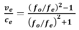
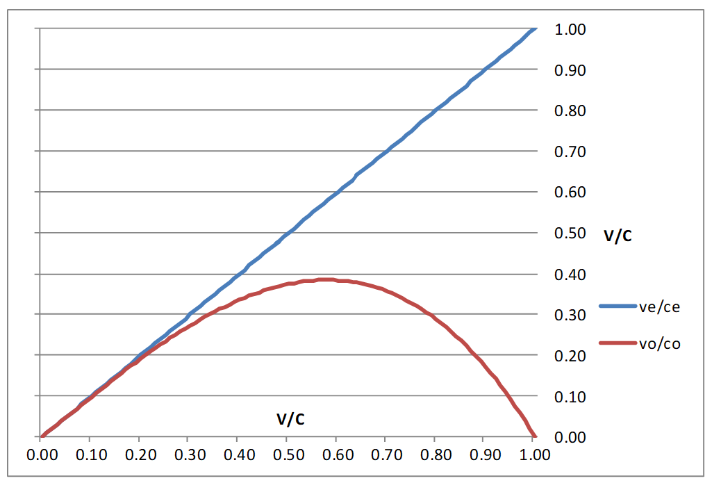
Note: The solution is for v_e , the local or apparent velocity. Conversion to v₀ produces the actual velocity compared to the observer. The clock of the emitter in motion is always slower than the observer’s clock. The actual velocity is always less than the local or apparent velocity.

The present use of Doppler to determine velocity from the frequency ratio

Option (1) Text book model based is on the observer moving and the emitter stationary with redshift
(-v²¹): We know the earth is moving. When a model states it is based on a certain state or reference that is what it normally means! For some reason this model is not used?

Redshift, reverse action as per the energy solution above. The independent variable is the base or frame of reference in the denominator. It meets all of the tests for a redshift model and agrees with the redshift equation R model and transformed model above. Solve for ±v/c with the sign (direction) remaining with

This option is identical to the redshift equation (R) above and meets all the parameters for redshift. It is not presently used?

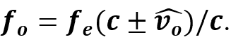
Option (2): Text book redshift model: Observer stationary and Emitter in motion = +v?²¹, is the present model being used when we know the Earth is a moving platform > 10⁶ miles/hr and do not know the status of E? 

This is not consistent with redshift but is with blueshift λ⤍(1→.5)range. If v=0→ f_o= 1 or f_o. The red direction was established at in Equation (R) and the transformed model. This equation is +v? The + velocity vector represents + blue direction not red. No matter what the state of the observer is, the observed shift cannot change. The different solutions are not compatible with SR (No preferred reference). The observer will see redshift as f_o < f_e in all cases the same as a SR solution.

Solving for v/c, f_o and f_e switch places. The denominator is f_o compared to f_e as per Textbook option (1).  This equation is based on f_o which is a different reference base than (1).
It is a blueshift model ( f_o > f_e ) , which is a bound relationship with v/c based on f_o rather than f_e .

 Solve for v/c:


Option 2 blueshift frequency:

Using the equation for the opposite shift inverts frequency to a wave calculation (z). This produces a hyperbolic curvature which exceeds c. This is discussed in the next section about z.

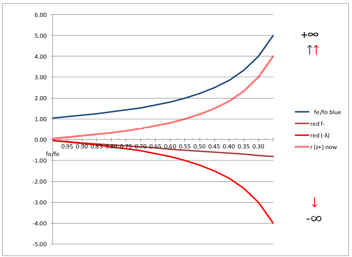
The use of z The definition of z is the fractional wave length change Δλ /λ_{(e or o)} caused by motion of an emitter.  The textbook choice of: + redshift z is based on the stationary observer

z=(λ₀-λ_e)/λ_e→λ_o/λ_e-1≅v/c ?

Since, λ_o→∞ this equation is not equal to ≅v/c and cannot be directly solved for v. If used for redshift it is hyperbolic curve to ∞. Distance and or velocity cannot be determined without a proper conversion. The z being used is not ≅ v/c. It only appears to be ≈ numerically accurate with the opposite sign at lower velocities but is mathematically incorrect. There is no solution using λ ratios to determine velocity in redshift because λ_o→∞ is in the numerator of the equation. The present calculation of z is a multiple of λ_o and not a fraction. The numerator is greater than the denominator.

Summary:
We have failed to integrate Special Relativity into astrophysics modeling which creates an issue with choice and accuracy. We have made incorrect choices using Doppler, which creates a hyperbolic solution for v. This results in models that violate the speed limit c. The assumed velocities of emitters have not been corrected to the observer’s frame. Some are replacing v with z in calculations. All of the errors are cumulative in the same direction, thus contribute to an illusion of a rapid expansion. The result is the Dark Energy theory (force with a string) to reconcile the observations. We need to get all of our determinations of velocity and distance as accurate as possible because we are projecting our models beyond the data. Keep in mind we can only do estimates ±. The error of measurement, distance and going back in time has a huge impact on the accuracy of our calculations.

Next month I will discuss issues with using standard candles to estimate distance.